A NUMERIC is not a BIGINT. Neither is a TIMESTAMP, a MAP, or — increasingly, and most
expensively — a VARIANT. Every engine in a modern data platform picked its own type system
under its own constraints, and those choices were reasonable in isolation. The trouble starts the
moment a value crosses a boundary: OLTP to CDC stream, stream to lakehouse table, lakehouse table
to warehouse, reverse ETL to serving datastore, K/V to RPC response. Somewhere on that path, a type mapping table — usually
undocumented, usually written once by whoever wired up the first connector — decides whether your
data survives the trip intact.
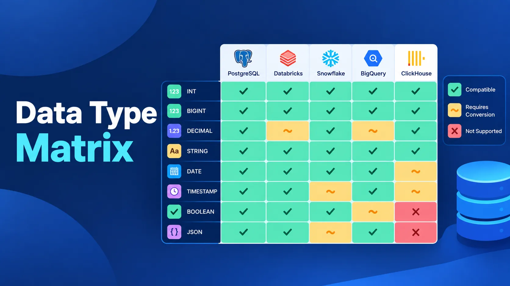
This post is a field guide to those mappings, and the companion spreadsheet is the reference you actually keep open in a tab. It covers nineteen systems people in this space touch daily — ClickHouse, Arrow, Parquet, Vortex, Spark SQL, Flink SQL, Iceberg, Delta Lake, Hudi, Paimon, Protobuf, Avro, Thrift, Postgres, Snowflake, BigQuery, StarRocks, DuckDB, and Trino — grouped into five families: numeric, string, date/time, binary, and composite/collection types. Postgres earns its spot for a practical reason: a large share of “different” engines in this space — CockroachDB, YugabyteDB, Amazon RDS/Aurora, Redshift’s client layer, and no small number of proprietary systems — speak the Postgres wire protocol and inherit its type vocabulary whether or not their storage engine has anything to do with Postgres internally, so its type system ends up being a de facto interchange dialect far beyond Postgres itself.
In addition, Postgres still has much richer types than most analytical databases, this introduces quite a bit edge cases (out of range/precision, composite/user_defined type).
Popularity wise, [Protobuf, Avro, Thrift, JSON] are the top RPC/API standard, but they have very limited types compared with SQL. SQL world is very divided without even a consensus of types. Easy-to-use data engines (such as Snowflake) go with relaxed/opaque types, but with the rise of Iceberg, the conversion to Iceberg become undeterministic (the on-the-fly type inference with limited sample records has many loose ends). Sub-second analytical engines (ClickHouse/StarRocks) and DataFusion have more precise types to take advantage of both storage and compute optimizations.
If you’d rather work from the file directly, download the workbook — five tabs of type-by-type mappings plus an Overview tab that counts, per engine and per category, how many of the fifty type concepts in the matrix each system actually has a dedicated type for. ClickHouse and Arrow are highlighted throughout for a reason: they come out at 48/50 and 41/50 respectively, comfortably ahead of most of the list (Thrift, at the other end, sits at 24/50 — not a criticism, just a much smaller, much older, much more deliberately minimal surface area). Every non-dash cell has a matching entry in the Conversion Notes column explaining the specific way that mapping bites you.
Two results in the Overview tab are worth calling out before you dig in, because they cut against
the obvious assumption. Postgres — the oldest system in this list by a couple of decades — ties
Arrow and DuckDB at 41/50, on the strength of native jsonb, uuid, ENUM, inet/cidr,
bit varying, arrays of any type including composite types, and an effectively unbounded NUMERIC.
BigQuery, by contrast, lands at a comparatively modest 34/50 despite being one of the two systems
this post’s newest worked example is about — and that’s not an oversight, it’s the whole point of
that example: BigQuery gets its expressiveness from composing a small number of types (STRUCT,
ARRAY, JSON) rather than adding new dedicated ones, which is a perfectly good design choice
until you’re the one deciding what a source column’s dedicated type should collapse into.
Table of contents
- Why this is a real problem and not a formatting nitpick
- Worked examples: where this actually bites
- The composite types worth slowing down for
- How to read the spreadsheet
Why this is a real problem and not a formatting nitpick
It’s tempting to treat type conversion as a solved problem — write a mapping table once, generate some codecs, move on. Three things make that not true in practice:
- The mapping isn’t always lossless, and the loss is often silent. A narrowing conversion that would throw in a strongly-typed language often just… happens, quietly, in a connector’s default cast logic. You find out when a downstream aggregate is wrong, not when the pipeline runs.
- Two types with the same name don’t always mean the same thing.
TIMESTAMPis the worst offender in this list (more below), butJSON,BINARY(n), andUNIONall name genuinely different concepts depending on which engine you’re standing in. - The newest, most interesting types are the least standardized. Variant, Geometry/Geography,
and Vector types are all mid-migration across this ecosystem right now, which means the matrix
entries for them are more likely to be stale in six months than the entries for
INT64. That’s not a flaw in the exercise — it’s the whole reason the exercise is worth doing.
Worked examples: where this actually bites
The timestamp that wasn’t naive
ClickHouse’s DateTime looks like a naive, zone-less timestamp — you write 2026-09-09 14:30:00
and that’s what comes back. It isn’t naive. Internally it’s a UTC instant plus a display
timezone attached to the column (or resolved from session_timezone if the column doesn’t specify
one). Two clients reading the same row with different session timezones see different wall-clock
strings for the identical stored instant.
Now migrate that column into a lakehouse table typed TIMESTAMP_NTZ (Delta) or Spark’s
TimestampNTZType — a genuinely naive type with no timezone concept attached at any layer. The
migration “succeeds”: the wall-clock string that ClickHouse happened to render for you at export
time gets baked in as if it had always been naive. Re-run the same export from a session with a
different timezone setting and you get a table with different values for the same underlying data.
The bug doesn’t show up in a schema diff — both columns are called TIMESTAMP — it shows up as an
inexplicable multi-hour skew that only appears for users in certain regions, discovered weeks later.
The fix is boring and always the same: pick one canonical representation (usually TIMESTAMP WITH TIME ZONE / timestamptz, i.e., an explicit UTC instant) as your interchange contract, and treat
“naive” columns as a lossy view generated from that contract, never as the source of truth for a
cross-system export.
The hash ID that went negative
If you’re generating surrogate keys with cityHash64 or similar inside ClickHouse — a common
pattern for high-cardinality dimension keys — you get a UInt64. Land that column, unchanged, into
Trino, Spark, or a plain Iceberg long (there is no unsigned integer type anywhere in that list),
and every value in the top half of the UInt64 range — anything at or above 2^63 — reads back as
a negative number. The join key still round-trips correctly as bits, so equi-joins between two
tables that both went through the same lossy cast still work. What breaks is anything that
compares, ranges, or sorts on the “ID” as a number, and any system that validates id > 0 as an
invariant.
The Overview tab’s numeric section makes this pattern easy to spot: UInt8/16/32 are almost
always safe to widen into the next signed type, but UInt64 has no safe signed landing spot short
of a DECIMAL/NUMBER — the matrix flags this explicitly rather than leaving it as a “well, it
depends” footnote.
The oneof that became three nullable columns
If your service boundary is gRPC — a fairly common choice, including as the schema source of truth
for internal service contracts — a Protobuf oneof gives you a real, compiler-checked closed union:
exactly one of N fields is set, enforced at (de)serialization time, not by convention. The moment
that message lands in a lakehouse table or a warehouse row, most engines in this matrix have
nothing that preserves the “exactly one” guarantee. The common outcome is a struct with one
nullable field per branch — which is a strictly weaker contract. Nothing stops all three fields
from being populated at once, or all three from being null, and nothing in the schema documents
that this was ever supposed to be exclusive. The two honest alternatives are DuckDB’s native
UNION type or Arrow’s Union type, both of which actually preserve the tag — worth reaching for
specifically when a oneof-shaped payload needs to survive a hop into analytics without quietly
downgrading its own contract.
Overloaded Type Problem
Because JSON has very limited data types, MongoDB is not included in the matrix. DynamoDB has even less types. But both can well represent the symptom of “overload”:
{ "createdAt": "2026-09-09T18:32:00.502Z" }
{ "createdAt": { "$date": "2026-09-09T18:32:00.502Z" } }

{ "createdAt": { "$date": { "$numberLong": "1788978720502" } } }

{ "createdAt": { "$date": 1788978720502 } }

{ "createdAt": { "$timestamp": { "t": 1788978720, "i": 502 } } }

{ "createdAt": 1788978720502 }  -- DynamoDB
{ "createdAt": 1788978720.502 }  -- TTL can only use epoch second
{ "createdAt": { "N": "1788978720" } }
{ "createdAt": { "S": "2026-09-09T18:32:00.502Z" } }
By reading the above formats, we can interprete “$date”, “$numberLong” and “$timestamp” as the TYPE key for the “oneOf”/“Union” type (Avro serialized JSON also has the similar style yet different keywords).
If we store them directly to Iceberg (even with Variant type), the columnar storage efficiency
gets ruined. When the flood of analytical queries come in, the reader SQLs will have to carry the
bloated CASE…WHEN…ELSE to deal with the overloaded createdAt. People copy-n-paste such a
snippet into thousands of different SQL scripts, but a new overload format is introduced by the
upstream serializer one day, then hundreds of data pipelines will fail in the next 24 hours.
When the ETL worker receives the JSON strings from a dump or CDC stream, it needs to check all the possible “known” overload structures first, then applies the corresponding function to convert the various inputs (even in the same batch/file) to a properly typed SQL/Iceberg/Arrow type.
The 76-digit decimal with nowhere to go
High precision decimal in Postgres (and Decimal256 shows up in ClickHouse) for exactly one
kind of workload: numbers that need more than 38 significant digits, which in practice means
token amounts on 18-decimal-precision chains, compounding-interest calculations carried out to
very high scale, or anything adjacent to DeFi/Crypto ledgers. Every SQL warehouse in this matrix —
Snowflake’s NUMBER, Trino’s and Spark’s DECIMAL, Iceberg’s decimal — caps out at 38 digits,
full stop, no configuration flag changes that. There is no lossless conversion here. The only
two honest options are rescaling before export (losing precision on purpose, deliberately, with
the loss documented) or splitting the value into a string or a pair of Decimal128s and
reassembling it downstream. Neither is something a generic connector does for you automatically,
which means this is a case where “just pipe it through Debezium/Fivetran/whatever and see what
happens” will produce a wrong number that looks plausible.
Precise types from an imprecise source: Snowflake to BigQuery
The examples so far are all “system A has a type system B doesn’t.” This one is different, and in some ways more common: it’s what happens when the source system deliberately doesn’t distinguish things the target system requires you to distinguish, and the deliberate choice was a good one for Snowflake’s own users.
Snowflake has exactly one numeric storage type. INT, INTEGER, BIGINT, NUMBER, and
DECIMAL(p,s) are all, under the hood, NUMBER(38,0) or some other precision/scale pair within the
same 38-digit family — Snowflake resolves the differences at the type-alias level, not the storage
level, and simply carries whatever precision and scale you declared (or the default of NUMBER(38,0)
if you declared none) as metadata on the column. That’s a genuinely good design inside Snowflake:
storage is uniform, arithmetic never needs an implicit numeric-family promotion, and nobody has to
pick between INT and BIGINT up front and guess wrong. It becomes a problem the moment you need
to leave, because Parquet and Iceberg don’t have a single opaque numeric type — they want you to
pick INT32, INT64, or a decimal(precision, scale) with real bytes-on-disk implications, and
Snowflake’s own metadata frequently doesn’t tell you which one is right. A column that has held
nothing but small order-quantity integers for its entire life can easily be declared NUMBER with
no explicit precision, which Snowflake silently resolves to NUMBER(38,0) — and an export tool
reading that metadata has no way to know the values never exceeded four digits. Two exporters see
that identical metadata and make two different, equally defensible choices: one plays it safe and
writes every such column as Parquet decimal(38,0) (correct, but 16 bytes per value where 4 would
do, and it forces every downstream reader to treat what is obviously an integer column as a decimal
type); the other samples the actual data and narrows it to INT32 (compact, but one unusually large
batch load away from a schema-evolution break).
The decimal(38,0)-everywhere choice, the conservative one, then runs into a second, sharper
problem on the way into BigQuery. BigQuery’s un-parameterized NUMERIC defaults to NUMERIC(38,9)
— 29 integer digits and 9 fractional digits, 38 total. A decimal(38,0) value from Parquet needs
all 38 digits before the decimal point. It does not fit in NUMERIC(38,9); it has to be promoted
to BIGNUMERIC, which costs meaningfully more storage and, at the time of writing, can’t be indexed
or clustered on in BigQuery the way NUMERIC can. So the “safe” choice at export time forces the
expensive choice at load time, for a column of small integers that never needed either — and this
is exactly the kind of decision that has to be made per-column, informed by the actual data, because
neither Snowflake’s metadata nor Parquet’s schema alone contains enough information to make it
automatically.
VARIANT compounds the same problem in the other type family. It’s common — and reasonable —
practice in Snowflake to land a whole nested payload (an API response, an event body) straight into
a VARIANT column rather than modeling it relationally up front, precisely because Snowflake makes
that cheap and the schema can stay fluid while the shape of the upstream data is still settling.
Exporting that column has three realistic outcomes, and picking between them is a judgment call, not
a mechanical translation: serialize it as an opaque JSON string (cheapest to write, but every reader
downstream — including BigQuery — now has to reparse it on every query, having thrown away whatever
typing Snowflake did have); infer a static STRUCT/ARRAY schema from a sample of the actual rows
(works fine until a row shows up with a field Snowflake never enforced as consistent — a key that’s
sometimes a number and sometimes a string is completely legal in a schemaless VARIANT column and
completely illegal in a BigQuery STRUCT); or land it in BigQuery’s native JSON type and only
carve out the handful of paths that are actually stable and hot into real typed columns alongside
it — which is the right answer, and also the one that requires someone who understands the data to
make per-field decisions, because it’s the same shredding tradeoff the Variant section below
describes, just without Iceberg v3’s shared metadata/value encoding to fall back on. There’s no
connector setting that makes this migration purely mechanical; “define the Parquet/Iceberg schema”
and “pick the BigQuery types” are two separate, judgment-heavy steps precisely because Snowflake’s
own flexibility — one number type, one variant type — is what made the source schema easy to write
and the target schema hard to infer.
The composite types worth slowing down for
The five-category structure of the matrix groups arrays, maps, and structs together with a handful of newer, harder types, because the newer ones are where actual translation complexity — not just width mismatches — lives.
Variant: a genuinely convergent moment
Snowflake’s VARIANT — a self-describing value stored as two binary fields, metadata (the field
names, types, and structure needed to interpret the payload) and value (the actual data) — is not
a new idea. What’s new, and worth calling out explicitly, is that in the last two years this exact
binary encoding has been adopted essentially verbatim by Parquet, Apache Iceberg (as a core v3
type), Delta Lake, Apache Hudi, and — as of the last release cycle — Apache Paimon. That’s a real
convergence in an ecosystem that otherwise agrees on almost nothing at the composite-type level,
and it’s worth trusting: a Variant column written by Spark 4 and read by an Iceberg-V3-aware
engine is working with the same wire format, not just a similarly-named one.
Where it still gets complicated is shredding. The unshredded form is simple and portable — a
metadata blob and a value blob, full stop — but it means every query that touches even one field of
a Variant column has to deserialize the whole value. Shredding pulls consistently-present,
consistently-typed paths (a location field, a timestamp field) out into real, typed
typed_value columns alongside the catch-all value, so a predicate on payload.location can be
pushed down and evaluated without touching the rest of the document. Every engine in the convergent
group is implementing shredding on its own timeline. The practical consequence: two Variant
columns can be byte-for-byte identical in their unshredded encoding and still perform
completely differently under a selective query, purely because one engine’s writer shredded the
hot paths and the other’s didn’t yet. If you’re evaluating Variant support in a table format or
engine, “does it support Variant” is the wrong question — “does it shred, and which paths” is the
one that determines whether it’s actually usable at scale.
Geometry and Geography: not the same math, and that’s the point
Iceberg v3’s geometry and geography types (with parallel additions in Parquet, and native
support in Snowflake and ClickHouse’s geo family) look, at first glance, like two names for the
same thing: both are Well-Known-Binary-encoded shapes. They aren’t interchangeable, and treating
one as the other doesn’t produce a slightly-imprecise answer — it produces a wrong one.
Geometry is planar: coordinates are Cartesian (x, y) pairs, distances are Euclidean, and there’s
an explicit coordinate reference system (defaulting to OGC:CRS84) that defines what those
coordinates mean. Geography is spherical: coordinates are longitude/latitude on a model of the
Earth’s actual curved surface, and — critically — the format requires you to declare which
edge-interpolation algorithm turns two points into a line between them (SPHERICAL, VINCENTY,
THOMAS, ANDOYER, or KARNEY, each a different approximation of geodesic distance with a
different accuracy/cost tradeoff). Compute a “distance between two points” or a “does this polygon
contain this point” query using planar math on data that’s actually geographic, and the error grows
with the size of the region — negligible for a few city blocks, meaningfully wrong at
country-or-larger scale.
This is also, unusually for this list, a case where the standardization work is happening in the
open right now: the Iceberg v3 geospatial spec was co-designed with the Apache Sedona project and
validated in production against Snowflake’s existing GEOMETRY/GEOGRAPHY implementation before
being generalized into the open table-format spec. That’s worth knowing if you’re deciding whether
to trust it yet — it’s not a hastily-added feature flag, but the matrix still shows it as absent
from most of the engines on this list (Spark’s own core SQL still has no native geometry type;
you’re relying on Apache Sedona or an Iceberg-v3 read path either way), so plan for a WKB-blob-plus-
documented-CRS-convention fallback anywhere the native type hasn’t landed yet.
How to read the spreadsheet
Each of the five category tabs has one row per type concept and one column per engine. A dash
means “no dedicated type” — not “impossible to represent” — and the Conversion Notes column
(intentionally wide, wrapped, and the last column on every tab) says what the actual workaround is
and what it costs. The Overview tab turns the whole matrix into COUNTIF formulas against each
category tab, so the type-count comparisons update automatically if you extend the data — useful if
you want to fork this for a system that isn’t on the list yet.
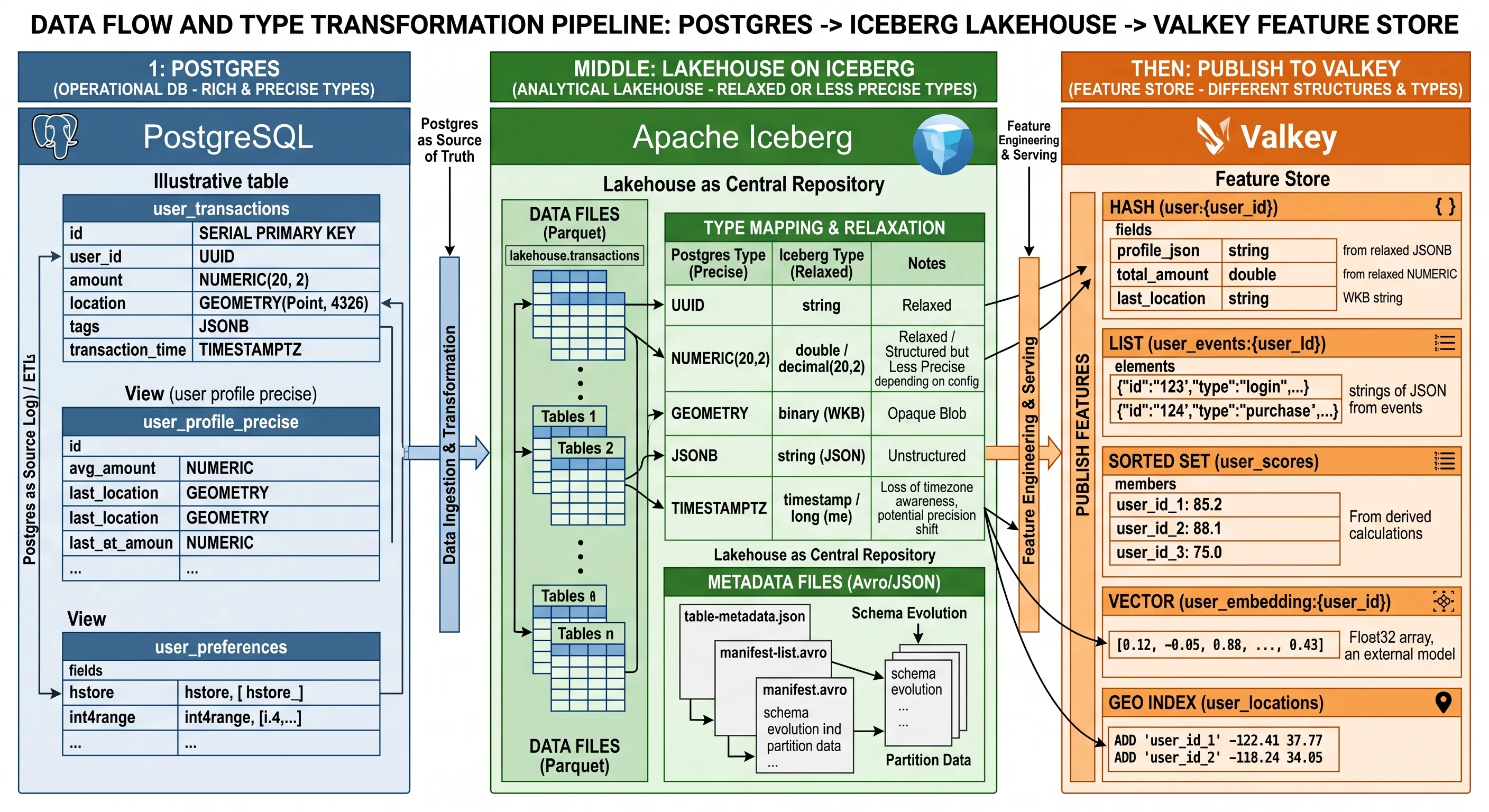
Companion workbook: data-type-matrix. Corrections and additions welcome — several of the newest rows (Variant shredding timelines, native Geometry/Geography support, Vector type constraints) are moving targets and this post will be updated as they settle.